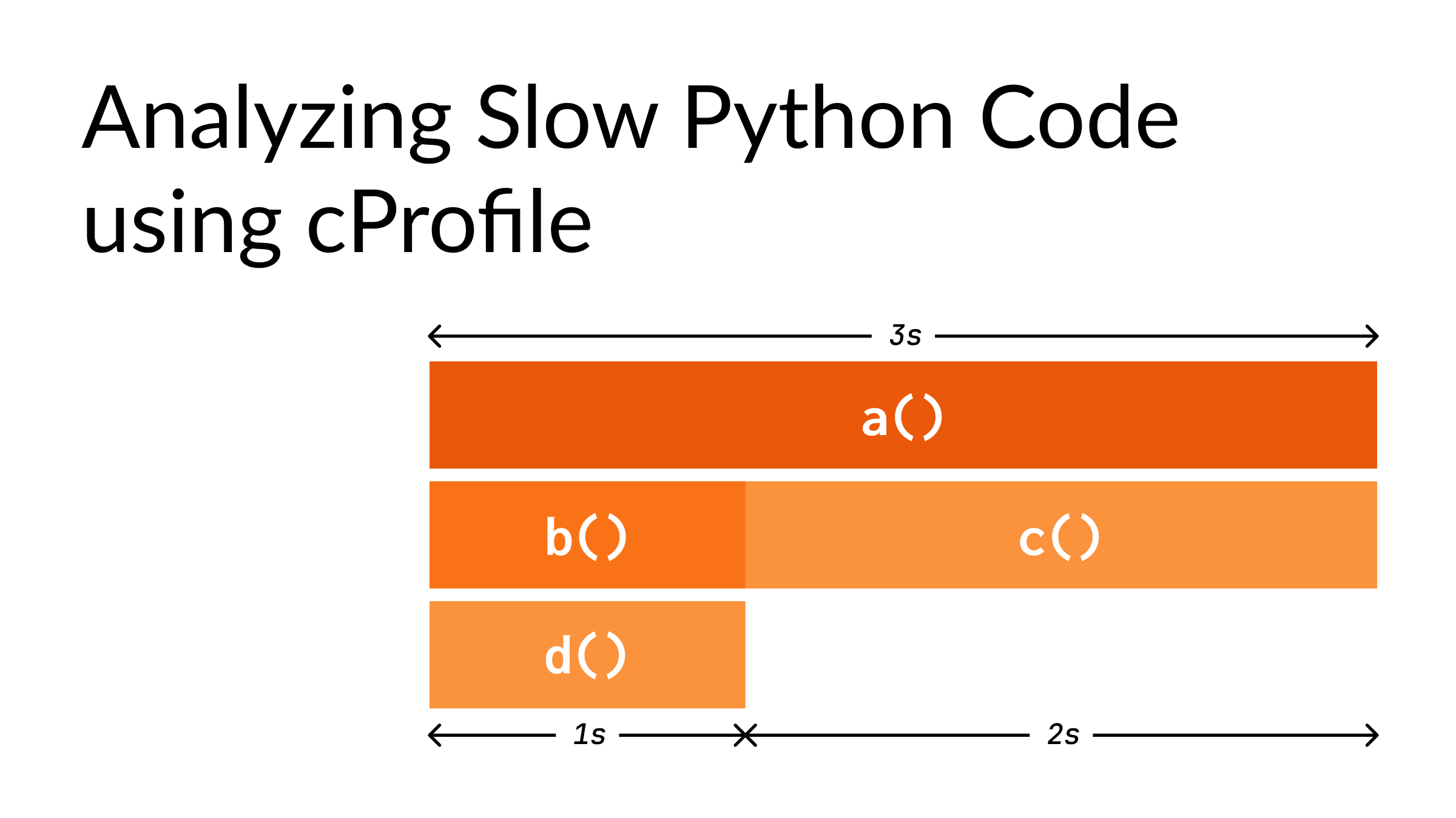
Analyzing Slow Python Code using cProfile
Python is widely considered to be a slow language. However it’s slow only when compared to other fast languages. I’d argue it’s a perfectly fine language for most applications - It’s very easy to learn which makes it ideal for teams with junior developers and its simplicity allows developers to focus on solving problems instead of worrying about low level details.
So it’s no surprise when lot of companies start with Python in the beginning. Most companies fail, so might as well fail faster. If they succeed and start getting more customers, they start hitting the performance limitations of Python. At this point, they can throw away the code and rewrite in a more performant language like Rust, but it’s better to profile your application and see where the bottlenecks are. Most of the time all you need to do is to find and fix these slow functions.
Before we jump into profiling, let’s build an intuition for flame graphs.
Let’s start with a simple example:
# test.py
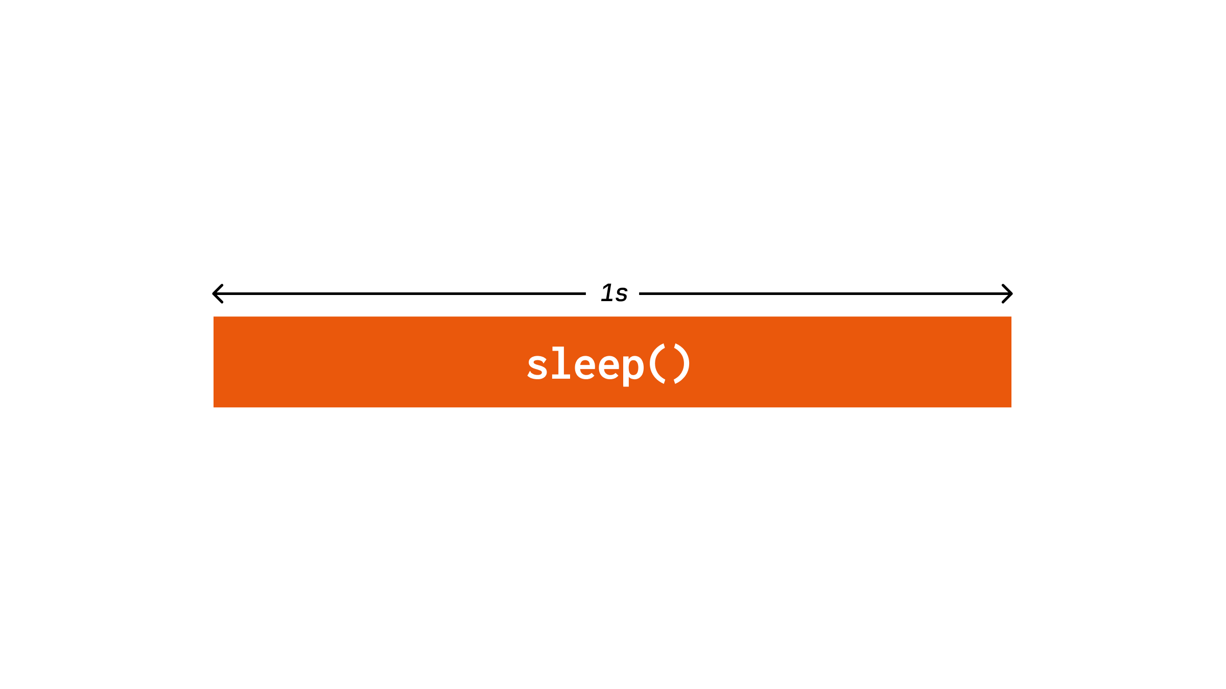
from time import sleep
sleep(1)This script will take 1 second to run and it can be visualized as:
The horizontal bar indicates the amount of time. Let’s add a function around it:
# test.py
from time import sleep

def a():
    sleep(1)

a()
This would look like:
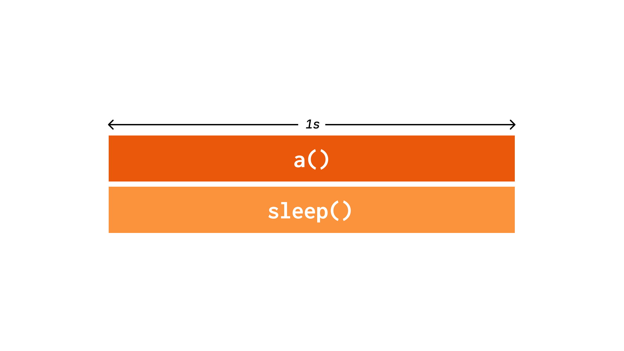
Notice how even though a() doesn’t do anything except call sleep(), it still has the same length. This is because these bars are cumulative, that is they add up. Which makes sense as the time spent on a function should be the total time of all the functions it calls and so on. In cProfile, this is called as cumtime. The time spent only on a() which is close to 0 is known as total time or tottime.
Let’s look at a one more example:
# test.py
from time import sleep

def a():
    sleep(1)
    b()
    sleep(1)

def b():
    sleep(1)

a()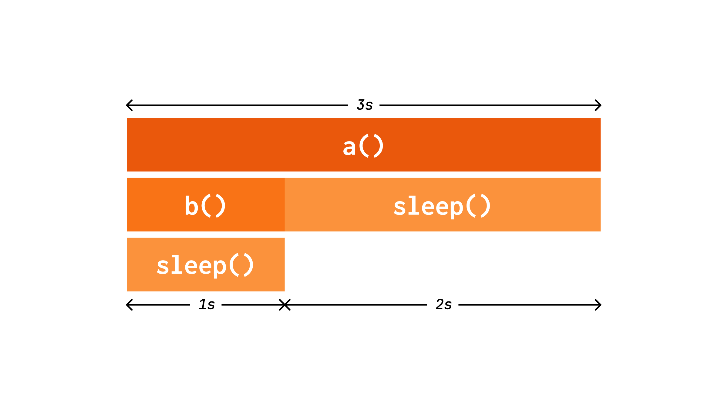
Here we can see that even though call sleep() twice in a(), it’s been collapsed into a single bar. This is because in real programs, there’ll be thousands or millions of calls to a function which can’t all be represented separately.
Since sleep() is called 3 times, the ntimes value in cProfile would be 3. We know the tottime and cumtime, and these sum up the time taken for all calls. To get a percall value for a function, we need to divide tottime and cumtime by ntimes . For example, here since tottime for sleep() is 3s, the percall value for tottime would be 1.
This should be sufficient to understand the flame graphs. Note that in the above examples, I used a variation of flame graphs called icicle graphs which are same as flame graphs but upside down.
To profile the above code, we need to make changes as follows:
# test.py
from time import sleep
+ import cProfile, pstats

def a():
    sleep(1)
    b()
    sleep(1)

def b():
    sleep(1)

+ profiler = cProfile.Profile()
+ profiler.enable()
a()
+ profiler.disable()
+ stats = pstats.Stats(profiler)
+ stats.dump_stats("./cProfile.stats")
+ stats.print_stats()
This can be run as python3 test.py and you’ll see the following results in the terminal:
$ python3 test.py
         6 function calls in 3.004 seconds

   Random listing order was used

   ncalls  tottime  percall  cumtime  percall filename:lineno(function)
        3    3.004    1.001    3.004    1.001 {built-in method time.sleep}
        1    0.000    0.000    0.000    0.000 {method 'disable' of '_lsprof.Profiler' objects}
        1    0.000    0.000    3.004    3.004 /home/user/test.py:5(a)
        1    0.000    0.000    1.001    1.001 /home/user/test.py:10(b)
You should be able to make sense of the values in above table.
Let’s use a tool called SnakeViz to visualize this. Install the tool and run:
pip install snakeviz
snakeviz cProfile.stats
You should see the page opened in the browser:
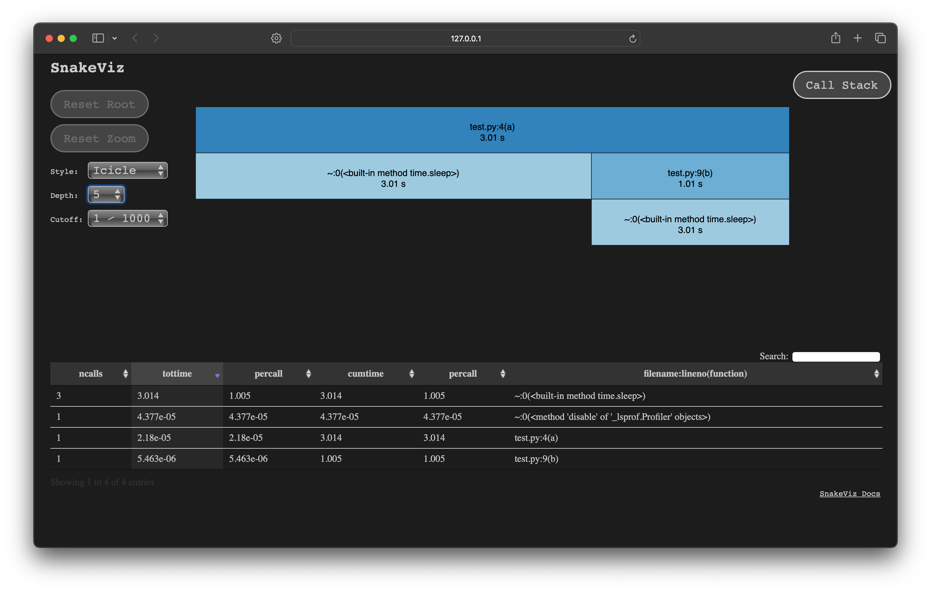
This is very similar to our diagrams above. Note that sleep() gets merged into a single row at the bottom which shows its tottime.